A simple yet powerful library, dedicated to the static analysis of electrical distribution networks
Features

Meshed Networks
Roseau Load Flow is perfectly suited for the study of meshed networks.

Multiple Phases
Single-phase, two-phase, three-phase, or more: with Roseau Load Flow, the number of phases matters little. Thanks to its generality, the library is adapted to the simulation of exotic cases, such as American “split-phases.”

Unbalanced Loads and Faults
Roseau Load Flow is designed to accurately model electrical unbalance situations. With us, no simplification like Kron reduction!
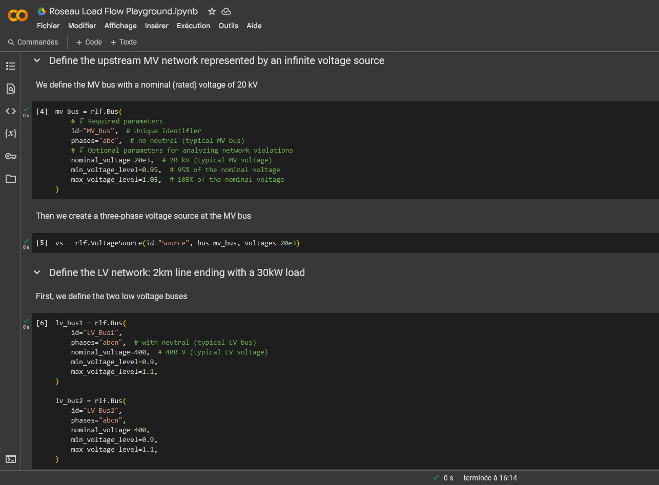
Roseau Load Flow in your web browser
The simplest way is to try it
Interested in our API? Try it immediately in your browser!
Thanks to this tutorial integrated into a Google Colab notebook, you don’t need to install Python on your machine, nor read the documentation: we guide you step by step, all you have to do is execute the code.
Follow our examples, modify them, and create new ones, in just a few clicks!
A User-Centric API
User Experience
1
Object-Oriented Modeling
2
Catalogs
Lines, transformers, loads, or even complete networks: everything is at your disposal for quick onboarding!
3
Flexible Loads
Easily integrate flexible loads by defining their P(U) and/or Q(U) controls and apparent power limits.
4
Generality
Model asymmetrical networks such as American “split-phase” systems.
5
Import and Export Functions
Roseau Load Flow facilitates your imports from DGS and OpenDSS formats and allows exports in a transparent JSON format.
6
Google Colab
Roseau Load Flow is perfectly usable in an online notebook such as Google Colab.
7
Documentation
Roseau Load Flow is a concise and well-documented Python API! Our models are precisely described within it.
8
Physical Units
Work in your preferred unit system and easily manage conversions to avoid errors.
Quality
A Robust and Accurate Load Flow API
We leveraged our expertise in optimization and applied mathematics to develop a power flow solver that is unique in the world.
High-Performance Algorithms
Roseau Load Flow relies on a Newton-Raphson type algorithm optimized with a Goldstein and Price function, ensuring faster and more stable convergence than a simple fixed-point algorithm.
Unsimplified Physical Models
The performance of our algorithms allows us to solve complete physical models. We apply no simplifications, such as Kron reduction, to guarantee you the most precise result.
An Extensible Solver
Roseau Load Flow is entirely modular, and the component model is generic. It's possible to define any new object by simply providing its equations, making the solver ideal for modeling atypical components (flexible loads, balancers, etc.).
Benchmark
Compare the different load flow solvers
| Power Factory | OpenDSS | pandapower | Roseau Load Flow | |
| User-Friendliness | ✕ | ✕ | 🗸 | 🗸 |
| Scalability | 🗸? | 🗸? | ≈ | 🗸 |
| Customization | ✕ | ✕ | 🗸 | ≈ |
| Automation | ≈ | ≈ | 🗸 | 🗸 |
| Accuracy of imbalance modeling | ≈? | 🗸 | ✕ | 🗸 |
| Documentation and grid data | ≈ | ≈ | 🗸 | 🗸 |
| Technical support | ✕ | ✕ | ≈ | 🗸 |
Licences
Licenses for Every Need
Free
forever!
- Public key
- Compatible with Google Colab
- Access to all features
- Unlimited calculations
- Up to 10 nodes
Research and Education
to be renewed annually
- Private key
- Access to all features
- Unlimited calculations
- Unlimited nodes
- Up to 3 devices
Commerciale
Contact Us
- Private key
- Access to all features
- Unlimited calculations
- Unlimited nodes
- Up to 3 devices
FAQ
We Answer Your Questions
About Licenses
Roseau Technologies originated from the academic world, and we remain deeply committed to research and education. We developed Roseau Load Flow for our internal needs because existing commercial solvers didn’t meet our quality and flexibility requirements. We believe Roseau Load Flow is currently the best load flow calculation solver available, and it feels natural to share this incomparable tool with our fellow researchers and educators!
Are you a researcher looking to support this initiative? Discover how!
We’re delighted to hear that Roseau Load Flow is working well for you!
To help us out, please spread the word! You can follow the Roseau Load Flow GitHub repository, tell other researchers and students in your lab about us, and most importantly, cite us in publications where you use our library.
Roseau Load Flow isn’t free for commercial use. If you’re interested in using Roseau Load Flow for your business activities, please contact us!
Roseau Load Flow is not Open Source.
Specifically, the C++ core of the solver is not distributed under an open license.
Electrotechnics and Solvers
Lorem ipsum dolor sit amet, consectetur adipisicing elit. Optio, neque qui velit. Magni dolorum quidem ipsam eligendi, totam, facilis laudantium cum accusamus ullam voluptatibus commodi numquam, error, est. Ea, consequatur.
Lorem ipsum dolor sit amet, consectetur adipisicing elit. Optio, neque qui velit. Magni dolorum quidem ipsam eligendi, totam, facilis laudantium cum accusamus ullam voluptatibus commodi numquam, error, est. Ea, consequatur.
Lorem ipsum dolor sit amet, consectetur adipisicing elit. Optio, neque qui velit. Magni dolorum quidem ipsam eligendi, totam, facilis laudantium cum accusamus ullam voluptatibus commodi numquam, error, est. Ea, consequatur.
Lorem ipsum dolor sit amet, consectetur adipisicing elit. Optio, neque qui velit. Magni dolorum quidem ipsam eligendi, totam, facilis laudantium cum accusamus ullam voluptatibus commodi numquam, error, est. Ea, consequatur.
Documentation
Thank you for your interest!
To get started with Roseau Load Flow, we invite you to
follow the dedicated tutorial.
You can also browse the Notebook dedicated to getting started with the library.
We’d be delighted to answer your questions! We invite you to open a ticket on the Roseau Load Flow GitHub repository. This way, the answer will be available to all API users.